Step response

[bonfire]

Step response


The step response of a system in a given initial state consists of the time evolution of its outputs when its control inputs are Heaviside step functions. In electronic engineering and control theory, step response is the time behaviour of the outputs of a general system when its inputs change from zero to one in a very short time. The concept can be extended to the abstract mathematical notion of a dynamical system using an evolution parameter.


From a practical standpoint, knowing how the system responds to a sudden input is important because large and possibly fast deviations from the long term steady state may have extreme effects on the component itself and on other portions of the overall system dependent on this component. In addition, the overall system cannot act until the component's output settles down to some vicinity of its final state, delaying the overall system response. Formally, knowing the step response of a dynamical system gives information on the stability of such a system, and on its ability to reach one stationary state when starting from another.







Time domain versus frequency domain

Instead of frequency response, system performance may be specified in terms of parameters describing time-dependence of response. The step response can be described by the following quantities related to its time behavior,

• overshoot
• rise time
• settling time
• ringing

In the case of linear dynamic systems, much can be inferred about the system from these characteristics. Below the step response of a simple two-pole amplifier is presented, and some of these terms are illustrated.
[edit] Step response of feedback amplifiers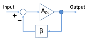


Figure 1: Ideal negative feedback model; open loop gain is AOL and feedback factor is β.


This section describes the step response of a simple negative feedback amplifier shown in Figure 1. The feedback amplifier consists of a main open-loop amplifier of gain AOL and a feedback loop governed by a feedback factor β. This feedback amplifier is analyzed to determine how its step response depends upon the time constants governing the response of the main amplifier, and upon the amount of feedback used.
[edit] Analysis

A negative feedback amplifier has gain given by (see negative feedback amplifier):
where AOL = open-loop gain, AFB = closed-loop gain (the gain with negative feedback present) and β = feedback factor. The step response of such an amplifier is easily handled in the case that the open-loop gain has two poles (two time constants, τ1, τ2), that is, the open-loop gain is given by:
with zero-frequency gain A0 and angular frequency ω = 2πf, which leads to the closed-loop gain:
  •  
Figure 2: Conjugate pole locations for a two-pole feedback amplifier; Re(s) = real axis and Im(s) = imaginary axis.


The time dependence of the amplifier is easy to discover by switching variables to s = jω, whereupon the gain becomes:
  •   The poles of this expression (that is, the zeros of the denominator) occur at:
which shows for large enough values of βA0 the square root becomes the square root of a negative number, that is the square root becomes imaginary, and the pole positions are complex conjugate numbers, either s+ or s−; see Figure 2:
with
and
Using polar coordinates with the magnitude of the radius to the roots given by |s| (Figure 2):
and the angular coordinate φ is given by:
Tables of Laplace transforms show that the time response of such a system is composed of combinations of the two functions:
e − ρtcos(μt), which is to say, the solutions are damped oscillations in time. In particular, the unit step response of the system is:[1]
Notice that the damping of the response is set by ρ, that is, by the time constants of the open-loop amplifier. In contrast, the frequency of oscillation is set by μ, that is, by the feedback parameter through βA0. Because ρ is a sum of reciprocals of time constants, it is interesting to notice that ρ is dominated by the shorter of the two.
[edit] Results


Figure 3: Step-response of a linear two-pole feedback amplifier; time is in units of 1/ρ, that is, in terms of the time constants of AOL; curves are plotted for three values of mu = μ, which is controlled by β.




Figure 3 shows the time response to a unit step input for three values of the parameter μ. It can be seen that the frequency of oscillation increases with μ, but the oscillations are contained between the two asymptotes set by the exponentials [ 1 − exp (−ρt) ] and [ 1 + exp(−ρt) ]. These asymptotes are determined by ρ and therefore by the time constants of the open-loop amplifier, independent of feedback.
The phenomena of oscillation about final value is called ringing. The overshoot is the maximum swing above final value, and clearly increases with μ. Likewise, the undershoot is the minimum swing below final value, again increasing with μ. The settling time is the time for departures from final value to sink below some specified level, say 10% of final value.
The dependence of settling time upon μ is not obvious, and the approximation of a two-pole system probably is not accurate enough to make any real-world conclusions about feedback dependence of settling time. However, the asymptotes [ 1 − exp (−ρt) ] and [ 1 + exp (−ρt) ] clearly impact settling time, and they are controlled by the time constants of the open-loop amplifier, particularly the shorter of the two time constants. That suggests that a specification on settling time must be met by appropriate design of the open-loop amplifier.
The two major conclusions from this analysis are:

1. Feedback controls the amplitude of oscillation about final value for a given open-loop amplifier and given values of open-loop time constants, τ1 and τ2.
2. The open-loop amplifier decides settling time. It sets the time scale of Figure 3, and the faster the open-loop amplifier, the faster this time scale.

As an aside, it may be noted that real-world departures from this linear two-pole model occur due to two major complications: first, real amplifiers have more than two poles, as well as zeros; and second, real amplifiers are nonlinear, so their step response changes with signal amplitude.

Figure 4: Step response for three values of α. Top: α = 4; Center: α = 2; Bottom: α = 0.5. As α is reduced the pole separation reduces, and the overshoot increases.


[edit] Control of overshoot

How overshoot may be controlled by appropriate parameter choices is discussed next.
Using the equations above, the amount of overshoot can be found by differentiating the step response and finding its maximum value. The result for maximum step response Smax is:[2]
The final value of the step response is 1, so the exponential is the actual overshoot itself. It is clear the overshoot is zero if μ = 0, which is the condition:
This quadratic is solved for the ratio of time constants by setting x = ( τ1 / τ2 )1 / 2 with the result
Because β A0 >> 1, the 1 in the square root can be dropped, and the result is
In words, the first time constant must be much larger than the second. To be more adventurous than a design allowing for no overshoot we can introduce a factor α in the above relation:
and let α be set by the amount of overshoot that is acceptable.
Figure 4 illustrates the procedure. Comparing the top panel (α = 4) with the lower panel (α = 0.5) shows lower values for α increase the rate of response, but increase overshoot. The case α = 2 (center panel) is the maximally flat design that shows no peaking in the Bode gain vs. frequency plot. That design has the rule of thumb built-in safety margin to deal with non-ideal realities like multiple poles (or zeros), nonlinearity (signal amplitude dependence) and manufacturing variations, any of which can lead to too much overshoot. The adjustment of the pole separation (that is, setting α) is the subject of frequency compensation, and one such method is pole splitting.
[edit] Control of settling time

The amplitude of ringing in the step response in Figure 3 is governed by the damping factor exp ( −ρ t ). That is, if we specify some acceptable step response deviation from final value, say Δ, that is:
this condition is satisfied regardless of the value of β AOL provided the time is longer than the settling time, say tS, given by:[3]
where the approximation τ1 >> τ2 is applicable because of the overshoot control condition, which makes τ1 = αβAOL τ2. Often the settling time condition is referred to by saying the settling period is inversely proportional to the unity gain bandwidth, because 1/(2π τ2) is close to this bandwidth for an amplifier with typical dominant pole compensation. However, this result is more precise than this rule of thumb. As an example of this formula, if Δ = 1/e4 = 1.8 %, the settling time condition is tS = 8 τ2.
In general, control of overshoot sets the time constant ratio, and settling time tS sets τ2.[4][5] [6]
[edit] Phase margin


Figure 5: Bode gain plot to find phase margin; scales are logarithmic, so labeled separations are multiplicative factors. For example, f0 dB = βA0 × f1.


Next, the choice of pole ratio τ1/τ2 is related to the phase margin of the feedback amplifier.[7] The procedure outlined in the Bode plot article is followed. Figure 5 is the Bode gain plot for the two-pole amplifier in the range of frequencies up to the second pole position. The assumption behind Figure 5 is that the frequency f0 dB lies between the lowest pole at f1 = 1/(2πτ1) and the second pole at f2 = 1/(2πτ2). As indicated in Figure 5, this condition is satisfied for values of α ≥ 1.
Using Figure 5 the frequency (denoted by f0 dB) is found where the loop gain βA0 satisfies the unity gain or 0 dB condition, as defined by:
The slope of the downward leg of the gain plot is (20 dB/decade); for every factor of ten increase in frequency, the gain drops by the same factor:[8][9]
The phase margin is the departure of the phase at f0 dB from −180°. Thus, the margin is:
Because f0 dB / f1 = βA0 >> 1, the term in f1 is 90°. That makes the phase margin:
In particular, for case α = 1, φm = 45°, and for α = 2, φm = 63.4°. Sansen[10] recommends α = 3, φm = 71.6° as a "good safety position to start with".
If α is increased by shortening τ2, the settling time tS also is shortened. If α is increased by lengthening τ1, the settling time tS is little altered. More commonly, both τ1 and τ2 change, for example if the technique of pole splitting is used.
As an aside, for an amplifier with more than two poles, the diagram of Figure 5 still may be made to fit the Bode plots by making f2 a fitting parameter, referred to as an "equivalent second pole" position.[11]
[edit] Formal mathematical description

Figure 4: Black box representation of a dynamical system, its input and its step response.


This section provides a formal mathematical definition of step response in terms of the abstract mathematical concept of a dynamical system : all notations and assumptions required for the following description are listed here.

• is the evolution parameter of the system, called "time" for the sake of simplicity,
• is the state of the system at time , called "output" for the sake of simplicity,
• is the dynamical system evolution function,
• is the dynamical system initial state,
• is the Heaviside step function

[edit] Nonlinear dynamical system

For a general dynamical system, the step response is defined as follows:
It is the evolution function when the control inputs (or source term, or forcing inputs) are Heaviside functions: the notation emphasizes this concept showing H(t) as a subscript.
[edit] Linear dynamical system

For a linear time-invariant black box, let for notational convenience: the step response can be obtained by convolution of the Heaviside step function control and the impulse response h(t) of the system itself